Tormod Landet

Articles in the Tech category

  1. Solving the Laplace equation with FEniCS

    I have found that explaining something is a good way to learn. As I am currently reading some books on the finite element method to refresh my rusting memories from math courses at university I thought it would be a good idea to write a summary of some of the basics. This post will explain how to use the finite element method and FEniCS for solving partial differential equations. FEniCS is a collection of tools for automated, efficient solution of partial differential equations using the finite element method.

    Introduction

    I will show how to apply FEniCS to a simple partial differential equation. I will also explain the solution method employed in the finite element method to solve the selected equation, the Laplace equation:

    \begin{equation*} \newcommand{\dif}{\mathrm{d}} \newcommand{\pdiff}[2]{\frac{\mathrm\partial#1}{\mathrm\partial#2}} \newcommand{\laplace}[1]{\nabla^2#1} \laplace{\phi} = 0 \end{equation*}

    When a fluid is incompressible, inviscid and the flow can be assumed to be irrotational then the Laplace equation shown above describes the fluid flow. The fluid velocities, \({\bf U} = (U_x, U_y, U_z)\), can be calculated from the velocity potential \(\phi\) as follows:

    \begin{equation*} U_x = \pdiff{\phi}{x} \qquad U_y = \pdiff{\phi}{x} \qquad U_z = \pdiff{\phi}{x} \end{equation*}

    Our domain, \(\Omega\), is a 2D square with \(x \in [0, 2]\) and \(y \in [0, 1]\). For the boundary conditions, let's say that we know the value of \(\phi\) at that the short boundaries and the normal derivative at the long edges is zero. The complete equation system can then be for example:

    \begin{align*} &\laplace{\phi} = 0 \\ \ \\ &\phi = -1.0 \quad &\text{on} \quad x = 0.0 \\ &\phi = +1.0 \quad &\text{on} \quad x = 2.0 \\ &\pdiff{\phi}{\bf n} = 42 \quad &\text{on} \quad \Gamma_L \\ \end{align*}

    where we define \(\Gamma_L\) to be the long edge boundaries \(y=0\) and \(y=1\). The normal vector on the boundary is \(\bf n\) and \(\pdiff{}{\bf n}\) is the normal derivative at the boundary. It is common to use \(\Omega\) to denote the domain and \(\Gamma\) to denote the boundary.

    Discretization

    Now, to solve the equation with boundary conditions we need a discretized domain. This can be created by using the FEniCS Python package dolfin like this:

    import dolfin as df
    
    start_x, end_x, n_elem_x = 0.0, 2.0, 4
    start_y, end_y, n_elem_y = 0.0, 1.0, 2
    
    mesh = df.RectangleMesh(start_x, start_y, end_x, end_y, n_elem_x, n_elem_y)
    

    Running df.plot(mesh) will show the following:

    The mesh

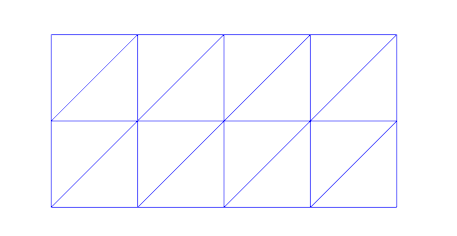
    An example mesh with triangular elements

    We discretize our domain \(\Omega\) into discrete elements and obtain \(\hat \Omega\). I will use the "hat" to denote discretized values. We use linear elements which means we will approximate the unknown function with piecewise linear functions, \(\phi \approx \hat \phi\). They look like this for a 1D domain with two elements and three vertices (nodes):

    Linear shape functions in 1D

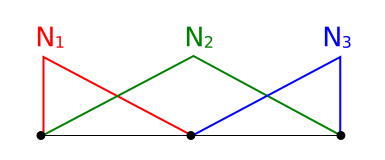
    1D domain with three shape functions, \(N_1(x)\), \(N_2(x)\) and \(N_3(x)\)

    We have one shape function \(N_i\) for each vertex in the mesh. The shape functions are equal to 1.0 at the corresponding vertex and 0.0 at all other vertices. In 2D a standard bi-linear shape function looks as follows:

    Linear shape function in 2D

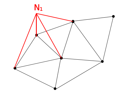
    2D domain with a bi-linear shape function shown for one of the vertices on the boundary

    Marking the boundaries

    We know how to make a mesh of the domain. We also need to tell FEniCS about the different parts of the boundary. We do this by giving the boundaries different unique integer numbers and marking the boundaries with a mesh function:

    # Each part of the mesh gets its own ID
    ID_LEFT_SIDE, ID_RIGHT_SIDE, ID_BOTTOM, ID_TOP, ID_OTHER = 1, 2, 3, 4, 5
    boundary_parts = df.MeshFunction("size_t", mesh, mesh.topology().dim()-1)
    boundary_parts.set_all(ID_OTHER)
    
    # Define the boundaries
    GEOM_TOL = 1e-6
    define_boundary(lambda x, on_boundary: on_boundary and x[0] < start_x + GEOM_TOL, boundary_parts, ID_LEFT_SIDE)
    define_boundary(lambda x, on_boundary: on_boundary and x[0] > end_x - GEOM_TOL, boundary_parts, ID_RIGHT_SIDE)
    define_boundary(lambda x, on_boundary: on_boundary and x[1] < start_y + GEOM_TOL, boundary_parts, ID_BOTTOM)
    define_boundary(lambda x, on_boundary: on_boundary and x[1] > end_y - GEOM_TOL, boundary_parts, ID_TOP)
    

    The define_boundary function is just a small utility I made to make it easier to mark the boundaries. Normally you need to create a class for each boundary and implement a method, inside, on this class. My function accepts a lambda expression which is used instead:

    def define_boundary(defining_func, boundary_parts, boundary_id):
        """
        Define a boundary
    
        - defining_func is used instead of the normal SubDomain inside method: defining_func(x, on_boundary)
        - boundary_parts is a MeshFunction used to distinguish parts of the boundary from each other
        - boundary_id is the id of the new boundary in the boundary_parts dictionary
        """
        class Boundary(df.SubDomain):
            def inside(self, x, on_boundary):
                return defining_func(x, on_boundary)
        boundary = Boundary()
        boundary.mark(boundary_parts, boundary_id)
        return boundary
    

    The solution method

    The simplest variant of the finite element method to describe is probably the Galerkin weighted residuals method. The core of the method is described below.

    The unknown function \(\phi\) is written as a sum of \(M\) shape functions and a set of unknown coefficients, \(a_i\). There is one unknown coefficient for each shape function:

    \begin{equation*} \hat \phi(x,y) = \sum_{i=0}^{M} a_i N_i(x,y) \end{equation*}

    Suppose we guess some coefficients \(a_i\). We can then integrate our trial function, \(\hat \phi\) over the domain, but since the discretization is not perfect we get a residual and not zero as the equation was supposed to give:

    \begin{equation*} \int_{\Omega} \laplace{\hat \phi} \ \dif \Omega = R \end{equation*}

    To be able to fix this and find some coefficients \(a_i\) that gives zero residual we need a set of equations. This is done by multiplying the above integral with a set of weighing functions, \(w_i(x,y)\). The number of weighting functions is equal to the number of unknowns, so we get a fully determined set of linear equations. In the Galerkin method the weighting functions are taken equal to the shape functions, \(N_i\) except that we do not include shape functions corresponding to vertices where we know the solution \(\phi(x,y)\) from the Dirichlet boundary conditions.

    We then get a set of \(M\) equations:

    \begin{equation*} \int_{\Omega} \laplace{\hat \phi} w_i \ \dif \Omega = 0 \end{equation*}

    which is the same as:

    \begin{equation*} \int_{\Omega} \laplace{\left(\sum_{j=0}^M a_j N_j\right)} N_i \dif \Omega = 0 \end{equation*}

    Since the integral will only be non-zero for vertices that are close in the mesh, i.e. \(N_i\) and \(N_j\) have some overlap, we end up with a quite sparse equation system. Very efficient solvers exist for the types of equation systems that come out of the Galerkin method.

    Solving the equation system with FEniCS

    In the standard finite element terminology our unknown function \(\phi\) is called the trial function and denoted \(u\) while the weighting function is called the test function and denoted \(v\). We switch to this terminology to be compatible with the FEniCS tutorial. We call this equation the weak form:

    \begin{equation*} \int_{\Omega} \laplace{(u)}\,v \ \dif \Omega = 0 \end{equation*}

    Before we are done we need to modify the equation a bit. As written it makes little sense since the Laplacian of the bi-linear function \(N_j(x,y)\) will always be zero. We modify our weak form by performing integration by parts. The formula for this in higher dimensions is:

    \begin{equation*} \int_\Omega \pdiff{f}{x_i}\,g \ \dif \Omega = \int_\Gamma f\,g\,n_i\ \dif \Gamma - \int_\Omega f \pdiff{g}{x_i} \ \dif \Omega \end{equation*}

    where \(n_i\) is the \(i\)-th component of the outwards normal vector on \(\Gamma\). I do not think I ever learned that at school? Maybe it's just my rusty memory, but thanks to Wikipedia we will not let lacking education and/or failing memory stop us, now will we? We get this when applying integration by parts to our integral:

    \begin{equation*} \int_\Omega \laplace{(u)}\,v \ \dif \Omega = \int_\Gamma \nabla(u)\,v\,n_i\ \dif \Gamma - \int_\Omega \nabla (u)\cdot\nabla(v) \ \dif \Omega \end{equation*}

    I guess now is the time for me to remember to mention that the test function \(v\) is always zero at the Dirichlet boundaries. Dirichlet boundaries are boundaries where we have Dirichlet boundary conditions, which means we know the value of \(\phi\), i.e. the short edges of our mesh in this case. No reason to have a weight function there, right? We now have the final expression for the weak form:

    \begin{align*} \int_{\Omega} \nabla u \cdot \nabla v \ \dif \Omega &= \int_{\Gamma_N} \laplace{(u)}\,v\,n_i\ \dif \Gamma_N \\ &= \int_{\Gamma_N} \pdiff{u}{\bf n}\,v\ \dif \Gamma_N \end{align*}

    The long edges were we prescribe the normal velocity (normal derivative of the velocity potential \(\phi\)) are now denoted \(\Gamma_N\) since this type of boundary condition is called a Neumann boundary condition.

    FEniCS understands equations such as the above and calls them forms. To describe the equations we use UFL, Uniform Form Language which is a Python API for defining forms. When interacting with FEniCS through Python we can use UFL through the dolfin package just like the mesh facilities. UFL can also be directly imported, import ufl.

    # Define a function space of bi-linear elements on our mesh
    V = df.FunctionSpace(mesh, 'Lagrange', 1)
    
    # The trial and test functions are defined on the bi-linear function space
    u = df.TrialFunction(V)
    v = df.TestFunction(V)
    
    # Our equation is defined as a=L. We only define what is inside the integrals, and the difference
    # between integrals over the domain and the boundary is whether we use dx or ds:
    #   - the term a contains both the trial (unknown) function u and the test function v
    #   - the term L contains only test function v
    a = df.inner(df.nabla_grad(u), df.nabla_grad(v))*df.dx
    L = df.Constant(42)*v*df.ds(ID_BOTTOM) + df.Constant(42)*v*df.ds(ID_TOP)
    

    This is basically all there is to solving the Laplace equation in FEniCS. The complete code can be seen below. The parts I have skipped explaining above are well explained in the FEniCS tutorial.

    Complete code

    The complete code can be found on Bitbucket. The resulting plot from running the code with FEniCS 1.3 is shown below:

    Plot of the result

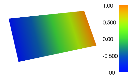
    Plot of the resulting \(\phi\) function

    If you have any questions to the above and how to use FEniCS you can ask here, but I would really recommend the FEniCS QA Forum where you will probably get better and faster answers.

  2. Creating a mesh in FEniCS

    I may end up doing a large project using FEniCS which is a collection of tools for automated, efficient solution of differential equations using the finite element method. While playing with implementing a simple solver for fluid flow in a tank by use of FEniCS to solve the Laplace equation I needed to create my own mesh in code.

    FEniCS is quite well documented, but I had to look at the source code for some of the mesh conversion routines to find out how to build a mesh from scratch. So, for posterity, here is a reimplementation of dolfin.RectangleMesh in a much more cumbersome (and flexible) way:

    import numpy
    import dolfin as df
    
    def create_mesh(length, height, nx, ny, show=False):
        """
        Make a square mesh manually
    
        Should give exactly the same results as using the built in dolfin.RectangleMesh() class
        """
        # The number of mesh entities
        nvert = nx*ny
        ncell = 2*(nx-1)*(ny-1)
    
        # Positions of the vertices
        xpos = numpy.linspace(0, length, nx)
        ypos = numpy.linspace(0, height, ny)
    
        # Create the mesh and open for editing
        mesh = df.Mesh()
        editor = df.MeshEditor()
        editor.open(mesh, 2, 2)
    
        # Add the vertices (nodes)
        editor.init_vertices(nvert)
        i_vert = 0
        for x in xpos:
            for y in ypos:
                editor.add_vertex(i_vert, x, y)
                i_vert += 1
    
        # Add the cells (triangular elements)
        # Loop over the vertices and build two cells for each square
        # where the selected vertex is in the lower left corner
        editor.init_cells(ncell)
        i_cell = 0
        for ix in xrange(nx-1):
            for iy in xrange(ny-1):
                # Upper left triangle in this square
                i_vert0 = ix*ny + iy
                i_vert1 = ix*ny + iy+1
                i_vert2 = (ix+1)*ny + iy + 1
                editor.add_cell(i_cell, i_vert0, i_vert1, i_vert2)
                i_cell += 1
    
                # Lower right triangle in this square
                i_vert0 = ix*ny + iy
                i_vert1 = (ix+1)*ny + iy+1
                i_vert2 = (ix+1)*ny + iy
                editor.add_cell(i_cell, i_vert0, i_vert1, i_vert2)
                i_cell += 1
    
        # Close the mesh for editing
        editor.close()
        print 'Created mesh with %d vertices and %d cells' % (nvert, ncell)
    
        if show:
            df.plot(mesh)
            df.interactive()
    
        return mesh
    

    If anyone finds this by searching the web for how to build a mesh programmatically in FEniCS/dolfin, then I hope the above was understandable. The documentation is quite good when you know that you need to search for the MeshEditor class ...

  3. Sorting images

    Once upon a time, back when I was using Windows at home, I had a useful small program that helped me sort through new pictures from my camera. I have forgotten the name of the program, but basically it allowed me to sort the good pictures from the bad in a fast and efficient manner so that the really bad ones could be deleted and the good ones could be separated, maybe for sharing with others.

    I have just been on a trip where I took quite some pictures. I could have gone over the pictures and manually copied the good ones into a separate folder for sharing with friends. This would have been a bit boring, but it would only have taken about five minutes. As a programmer I of course selected to optimize this task and spent some hours recreating the program I had once used. After a thousand trips or so I will come out ahead in terms of time spent!

    The program looks like this:

    Picster GUI

    I named it Picster, short for Picture Sorter. There is, of course, at least one other programs with that name already, but I cannot be bothered to find something better at the moment, It's just a script, after all. It is meant to be used from the keyboard, but there are also buttons for all possible actions (moving between images, categorizing images, and sorting images on disk based on category information).

    All of the GUI coding I do at work is scientific visualization, mostly using Python 2 and the wx library in some way. To try something slightly different I went with Python 3 and Qt for this program. I cannot really call myself an expert in Qt after only a couple of hours and the Picster code is probably not how a Qt expert would have written it, but it seems to work OK.

    From this brief encounter, Python Qt code seems to be a bit more verbose and tedious compared to wxPython. For example Qt/PySide is missing the nice init arguments, so all properties on an object must be set after creation through method calls. The API is not very pythonic with no use of Python properties as far as I understood. I am also missing docstring help on class and method name completion in Eclipse PyDev :-(

    Also missing as far as I understood is the wxPython ability to bind to any event from anywhere. To listen for keystrokes or window size change for example you must override virtual methods. For now I am happy with using wx at work. The Qt documentation that was rumored to be fabulous seems quite on the same level of the wx documentation as well.

    What I really liked about Qt was the Layouts which work almost exactly like Sizers in wx, except that they come with a sensible default spacing of widgets. This is a sore spot in laying out wx interfaces and always needs manual intervention to look good.

    Enough mostly unqualified statements about Qt vs. wx, here's the code for anyone interested in a picture sorting program. The code requires Python (probably works in versions 2 and 3, tested in 3.2) and PySide for Python bindings to Qt.

  4. Digital TV med CAM og kabel fra Canal Digital

    Jeg kjøpte meg en CA-modul (CAM/CI/Common Interface) på Lefdal etter at jeg hørte at Canal Digital endelig hadde godkjent en slik for bruk i kabelnettet. Dette betyr at hvis man har en avansert nok TV vil man kunne ta inn digital-TV på kabelnettet uten å kjøpe en stygg og dyr boks. I stedet må du kjøpe en dyr CA-modul (jeg betalte 1095,- kr) og 299,- i året i kortleie fra Canal Digital.

    Etter å ha kjøpt CAM-en ventet jeg litt under en uke før jeg fikk smart-kortet og en antennekabel fra Canal Digital. Så begynte moroa ... Det viser seg at TV-en min ikke er så glad i norsk digital kabel-TV (DVB-C). Jeg visste at den ikke var på lista over godkjente tv-er, men jeg hadde håpet at det skulle fungere (jeg var litt vag i butikken om hvilken modell jeg hadde så jeg fikk kjøpe CAM likevel). Etter litt undersøkelser viser det seg at det er mulig å få det til å fungere, men det er en del mikk.

    Bruksanvisning for Samsung A676:

    Sett inn CAM som beskrevet i bruksanvisningen. Hvis du går inn på CI-menyen vil det stå at abonnementet ditt er gyldig til 1990. Ikke bra. TV-en finner heller ingen kanaler. Løsningen er:

    • Sett språk til finsk på digital tv (ikke analog)
    • Velg manuelt søk og så kabel-tv
    • Velg symbol rate: 6950 kS/s og QAM 64 (256 på noen få frekvenser det 64 ikke fungerer. Disse sender HD tror jeg)
    • Punch inn alle frekvensene under. 80% funker med QAM 64 og resten fungerer (med noen få unntak) med QAM 256. Vet ikke om det er noe på disse eller om det er mulig å få inn noe mer. Det kan være at frekvensene er geografisk bestemt.

    Utdatert, se oppdatering nederst i posten

    • 290000 MHz (QAM 256)
    • 298000 MHz (QAM 256)
    • 306000 MHz
    • 314000 MHz
    • 322000 MHz
    • 330000 MHz (QAM 256)
    • 338000 MHz (QAM 256)
    • 346000 MHz
    • 354000 MHz
    • 362000 MHz
    • 370000 MHz
    • 378000 MHz
    • 386000 MHz
    • 394000 MHz
    • 402000 MHz
    • 410000 MHz
    • 418000 MHz
    • 426000 MHz
    • 434000 MHz (QAM 256)
    • 442000 MHz (tom?)
    • 450000 MHz
    • 458000 MHz
    • 466000 MHz (QAM 256)
    • 474000 MHz
    • 482000 MHz
    • 490000 MHz
    • 498000 MHz

    Data fra denne siden og denne. Det kan være det mangler noen frekvenser i lista. Det kan også være at du må søke gjennom alle frekvensene i ny og ne for å finne kanaler som er lagt til. Ikke helt ideelt altså.

    Etter en stund fikk jeg ikke lenger melding om at kanalene var sperret og CI-menyen viste at noe var oppdatert og at gyldighetsdatoen nå var 2010. Jeg fikk plutselig inn alle kanaler, men jeg tror dette er et lokkemiddel og at Canal+ etc blir blokkert etter en stund (når du er passelig hekta).

    Hvis du ikke gidder å kjøpe CAM til en tusenlapp før du finner ut om det fungerer for deg så skal det visst være mulig å gjøre alt det som står over også uten CAM. Du vil da få melding om at alle kanalene er blokkert, men du skal kunne søke dem inn og få opp TV-guide etc. Tv-guidene er jo også en av grunnene til å ha digital-TV. Samsung sin er litt (som i VELDIG) mye penere enn den som er på Canal Digital sine bokser. Hvorfor kjøpe boks til 3000 kr og TV til vesentlig mer når du ender opp med verdens styggeste menysystem? Det frister i alle fall ikke meg. Nå er det bare å håpe på at det kommer PVR-er som støtter CAM-modulen min og som har hakket lekrere menysystem enn boksen til Canal Digital. Jeg betaler gladelig litt mellomlegg for å slippe å ha noe så stygt i stua.

    Jeg har en Samsung LE40A676A1WXXE, men jeg tror det skal fungere på andre TV-er i samme serien, altså LExxA676. Disse er RiksTV-godkjent (DVB-T).

    Moralen er: kjøper du ny TV og vil være sikker på at det fungerer, sjekk lista over godkjente TV-er på www.canaldigital.no. Har du en A676 fra 2008/2009 så kan du få det til å fungere likevel, men det er en del mikk.

    Oppdatering november 2011: Nye frekvenser starter fra 290 med hopp på 8 som før. QAM 256 og symbolrate 6952 på de fleste. NRK ligger på 330/256/6952. Av og til kan det hjelpe å stå på en analog kanal før de digitale skal søkes inn, min TV finner av og til ikke kanaler på 330 før jeg gjør dette.

  5. Streaming audio from Spotify on Linux to Squeezebox

    I have tried the WaveInput route for SqueezeCenter, but due to a non-cooperative sound card and various problems with permissions related to SqueezeCenter running as a limited user I decided to go another route and stream sound from my Linux laptop via Icecast. If you want try using WaveInput and have the same problems with recording from the sound card as I have (it plain doesn't work with arecord and friends) there is a recipe here that might work for you.

    PulseAudio

    I need to use PulseAudio to get recording of sound played through the sound card to work as my Intel sound card refuses to allow me to record the sound directly. Luckily PulseAudio finally works OK for me now. I configured Wine with padsp winecfg and chose the OSS output driver for sound (ALSA works poorly at the moment). Now, run Spotify as padsp wine spotify.exe. Spotify should pop up in your PulseAudio Volume Control (pavucontrol) in the Playback tab.

    You need to define a PulseAudio sink that is different from the normal (output to PC speakers). I chose to call this sink spotify. Create the sink with the following command.

    pactl load-module module-null-sink sink_name=spotify

    The sink should pop up in the volume control under the Output Devices tab. Next, select this sink as the default for Spotify in the Playback tab (click the small down-arrow and choose Move Stream and then Null Output).

    Icecast

    You can run Icecast with a minimalistic configuration. I used the minimal example (/usr/share/doc/icecast2/icecast_minimal.xml.dist on Ubuntu) where I modified the passwords and the log directory (I set the log directory a directory where I have write permissions so that I can run Icecast as my own user). Start Icecast with

    icecast2 -c icecast.xml

    Gstreamer

    Finally I take the spotify PulseAudio sink and channel it to Icecast by use of Gstreamer. The magic command is (in one line).

    gst-launch-0.10 pulsesrc device=spotify.monitor ! audioconvert  ! vorbisenc bitrate=300000 ! oggmux ! shout2send ip=localhost port=8000 password=PASSWORD mount=stream.ogg

    The bit rate is set to the highest I could use without getting error messages (300kbps). I assume this is pretty transparent and does not degrade the 160kbps Spotify output much.

    Now tune your Squeezebox to URL http://ip-address-of-linux-machine:8000/stream.ogg. Modify the file name and port according to your configuration.

    Comments are disabled on this article due to problems with spam. Somehow spammers believe that link-spamming this page with praise for the article will send them lots of readers or google-points or something ...

    Update 2013: I no longer use this method and do not know if it still works or if there are better ways to do this now

« Page 2 / 3 »