Tormod Landet - Solving the Laplace equation with FEniCS

I have found that explaining something is a good way to learn. As I am currently reading some books on the finite element method to refresh my rusting memories from math courses at university I thought it would be a good idea to write a summary of some of the basics. This post will explain how to use the finite element method and FEniCS for solving partial differential equations. FEniCS is a collection of tools for automated, efficient solution of partial differential equations using the finite element method.

Introduction

I will show how to apply FEniCS to a simple partial differential equation. I will also explain the solution method employed in the finite element method to solve the selected equation, the Laplace equation:

\begin{equation*} \newcommand{\dif}{\mathrm{d}} \newcommand{\pdiff}[2]{\frac{\mathrm\partial#1}{\mathrm\partial#2}} \newcommand{\laplace}[1]{\nabla^2#1} \laplace{\phi} = 0 \end{equation*}

When a fluid is incompressible, inviscid and the flow can be assumed to be irrotational then the Laplace equation shown above describes the fluid flow. The fluid velocities, \({\bf U} = (U_x, U_y, U_z)\), can be calculated from the velocity potential \(\phi\) as follows:

\begin{equation*} U_x = \pdiff{\phi}{x} \qquad U_y = \pdiff{\phi}{x} \qquad U_z = \pdiff{\phi}{x} \end{equation*}

Our domain, \(\Omega\), is a 2D square with \(x \in [0, 2]\) and \(y \in [0, 1]\). For the boundary conditions, let's say that we know the value of \(\phi\) at that the short boundaries and the normal derivative at the long edges is zero. The complete equation system can then be for example:

\begin{align*} &\laplace{\phi} = 0 \\ \ \\ &\phi = -1.0 \quad &\text{on} \quad x = 0.0 \\ &\phi = +1.0 \quad &\text{on} \quad x = 2.0 \\ &\pdiff{\phi}{\bf n} = 42 \quad &\text{on} \quad \Gamma_L \\ \end{align*}

where we define \(\Gamma_L\) to be the long edge boundaries \(y=0\) and \(y=1\). The normal vector on the boundary is \(\bf n\) and \(\pdiff{}{\bf n}\) is the normal derivative at the boundary. It is common to use \(\Omega\) to denote the domain and \(\Gamma\) to denote the boundary.

Discretization

Now, to solve the equation with boundary conditions we need a discretized domain. This can be created by using the FEniCS Python package dolfin like this:

import dolfin as df

start_x, end_x, n_elem_x = 0.0, 2.0, 4
start_y, end_y, n_elem_y = 0.0, 1.0, 2

mesh = df.RectangleMesh(start_x, start_y, end_x, end_y, n_elem_x, n_elem_y)

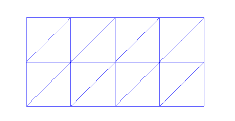
Running df.plot(mesh) will show the following:

An example mesh with triangular elements

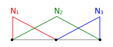
We discretize our domain \(\Omega\) into discrete elements and obtain \(\hat \Omega\). I will use the "hat" to denote discretized values. We use linear elements which means we will approximate the unknown function with piecewise linear functions, \(\phi \approx \hat \phi\). They look like this for a 1D domain with two elements and three vertices (nodes):

1D domain with three shape functions, \(N_1(x)\), \(N_2(x)\) and \(N_3(x)\)

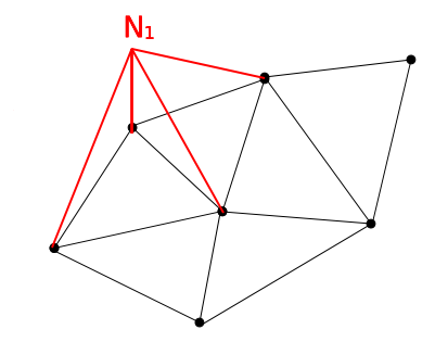
We have one shape function \(N_i\) for each vertex in the mesh. The shape functions are equal to 1.0 at the corresponding vertex and 0.0 at all other vertices. In 2D a standard bi-linear shape function looks as follows:

2D domain with a bi-linear shape function shown for one of the vertices on the boundary

Marking the boundaries

We know how to make a mesh of the domain. We also need to tell FEniCS about the different parts of the boundary. We do this by giving the boundaries different unique integer numbers and marking the boundaries with a mesh function:

# Each part of the mesh gets its own ID
ID_LEFT_SIDE, ID_RIGHT_SIDE, ID_BOTTOM, ID_TOP, ID_OTHER = 1, 2, 3, 4, 5
boundary_parts = df.MeshFunction("size_t", mesh, mesh.topology().dim()-1)
boundary_parts.set_all(ID_OTHER)

# Define the boundaries
GEOM_TOL = 1e-6
define_boundary(lambda x, on_boundary: on_boundary and x[0] < start_x + GEOM_TOL, boundary_parts, ID_LEFT_SIDE)
define_boundary(lambda x, on_boundary: on_boundary and x[0] > end_x - GEOM_TOL, boundary_parts, ID_RIGHT_SIDE)
define_boundary(lambda x, on_boundary: on_boundary and x[1] < start_y + GEOM_TOL, boundary_parts, ID_BOTTOM)
define_boundary(lambda x, on_boundary: on_boundary and x[1] > end_y - GEOM_TOL, boundary_parts, ID_TOP)

The define_boundary function is just a small utility I made to make it easier to mark the boundaries. Normally you need to create a class for each boundary and implement a method, inside, on this class. My function accepts a lambda expression which is used instead:

def define_boundary(defining_func, boundary_parts, boundary_id):
    """
    Define a boundary

    - defining_func is used instead of the normal SubDomain inside method: defining_func(x, on_boundary)
    - boundary_parts is a MeshFunction used to distinguish parts of the boundary from each other
    - boundary_id is the id of the new boundary in the boundary_parts dictionary
    """
    class Boundary(df.SubDomain):
        def inside(self, x, on_boundary):
            return defining_func(x, on_boundary)
    boundary = Boundary()
    boundary.mark(boundary_parts, boundary_id)
    return boundary

The solution method

The simplest variant of the finite element method to describe is probably the Galerkin weighted residuals method. The core of the method is described below.

The unknown function \(\phi\) is written as a sum of \(M\) shape functions and a set of unknown coefficients, \(a_i\). There is one unknown coefficient for each shape function:

\begin{equation*} \hat \phi(x,y) = \sum_{i=0}^{M} a_i N_i(x,y) \end{equation*}

Suppose we guess some coefficients \(a_i\). We can then integrate our trial function, \(\hat \phi\) over the domain, but since the discretization is not perfect we get a residual and not zero as the equation was supposed to give:

\begin{equation*} \int_{\Omega} \laplace{\hat \phi} \ \dif \Omega = R \end{equation*}

To be able to fix this and find some coefficients \(a_i\) that gives zero residual we need a set of equations. This is done by multiplying the above integral with a set of weighing functions, \(w_i(x,y)\). The number of weighting functions is equal to the number of unknowns, so we get a fully determined set of linear equations. In the Galerkin method the weighting functions are taken equal to the shape functions, \(N_i\) except that we do not include shape functions corresponding to vertices where we know the solution \(\phi(x,y)\) from the Dirichlet boundary conditions.

We then get a set of \(M\) equations:

\begin{equation*} \int_{\Omega} \laplace{\hat \phi} w_i \ \dif \Omega = 0 \end{equation*}

which is the same as:

\begin{equation*} \int_{\Omega} \laplace{\left(\sum_{j=0}^M a_j N_j\right)} N_i \dif \Omega = 0 \end{equation*}

Since the integral will only be non-zero for vertices that are close in the mesh, i.e. \(N_i\) and \(N_j\) have some overlap, we end up with a quite sparse equation system. Very efficient solvers exist for the types of equation systems that come out of the Galerkin method.

Solving the equation system with FEniCS

In the standard finite element terminology our unknown function \(\phi\) is called the trial function and denoted \(u\) while the weighting function is called the test function and denoted \(v\). We switch to this terminology to be compatible with the FEniCS tutorial. We call this equation the weak form:

\begin{equation*} \int_{\Omega} \laplace{(u)}\,v \ \dif \Omega = 0 \end{equation*}

Before we are done we need to modify the equation a bit. As written it makes little sense since the Laplacian of the bi-linear function \(N_j(x,y)\) will always be zero. We modify our weak form by performing integration by parts. The formula for this in higher dimensions is:

\begin{equation*} \int_\Omega \pdiff{f}{x_i}\,g \ \dif \Omega = \int_\Gamma f\,g\,n_i\ \dif \Gamma - \int_\Omega f \pdiff{g}{x_i} \ \dif \Omega \end{equation*}

where \(n_i\) is the \(i\)-th component of the outwards normal vector on \(\Gamma\). I do not think I ever learned that at school? Maybe it's just my rusty memory, but thanks to Wikipedia we will not let lacking education and/or failing memory stop us, now will we? We get this when applying integration by parts to our integral:

\begin{equation*} \int_\Omega \laplace{(u)}\,v \ \dif \Omega = \int_\Gamma \nabla(u)\,v\,n_i\ \dif \Gamma - \int_\Omega \nabla (u)\cdot\nabla(v) \ \dif \Omega \end{equation*}

I guess now is the time for me to remember to mention that the test function \(v\) is always zero at the Dirichlet boundaries. Dirichlet boundaries are boundaries where we have Dirichlet boundary conditions, which means we know the value of \(\phi\), i.e. the short edges of our mesh in this case. No reason to have a weight function there, right? We now have the final expression for the weak form:

\begin{align*} \int_{\Omega} \nabla u \cdot \nabla v \ \dif \Omega &= \int_{\Gamma_N} \laplace{(u)}\,v\,n_i\ \dif \Gamma_N \\ &= \int_{\Gamma_N} \pdiff{u}{\bf n}\,v\ \dif \Gamma_N \end{align*}

The long edges were we prescribe the normal velocity (normal derivative of the velocity potential \(\phi\)) are now denoted \(\Gamma_N\) since this type of boundary condition is called a Neumann boundary condition.

FEniCS understands equations such as the above and calls them forms. To describe the equations we use UFL, Uniform Form Language which is a Python API for defining forms. When interacting with FEniCS through Python we can use UFL through the dolfin package just like the mesh facilities. UFL can also be directly imported, import ufl.

# Define a function space of bi-linear elements on our mesh
V = df.FunctionSpace(mesh, 'Lagrange', 1)

# The trial and test functions are defined on the bi-linear function space
u = df.TrialFunction(V)
v = df.TestFunction(V)

# Our equation is defined as a=L. We only define what is inside the integrals, and the difference
# between integrals over the domain and the boundary is whether we use dx or ds:
#   - the term a contains both the trial (unknown) function u and the test function v
#   - the term L contains only test function v
a = df.inner(df.nabla_grad(u), df.nabla_grad(v))*df.dx
L = df.Constant(42)*v*df.ds(ID_BOTTOM) + df.Constant(42)*v*df.ds(ID_TOP)

This is basically all there is to solving the Laplace equation in FEniCS. The complete code can be seen below. The parts I have skipped explaining above are well explained in the FEniCS tutorial.

Complete code

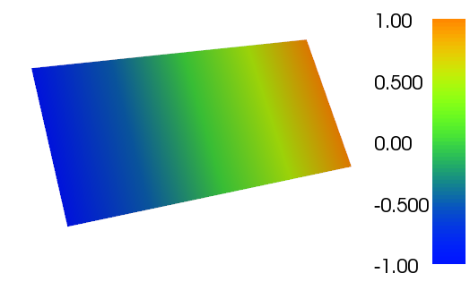
The complete code can be found on Bitbucket. The resulting plot from running the code with FEniCS 1.3 is shown below:

Plot of the resulting \(\phi\) function

If you have any questions to the above and how to use FEniCS you can ask here, but I would really recommend the FEniCS QA Forum where you will probably get better and faster answers.