Tormod Landet

Articles tagged with Code

  1. Ocellaris and my PhD project

    Ocellaris, the free surface two phase Navier-Stokes solver I have been building as a part of my PhD work at the Department of Mathematics at the University of Oslo is finally ready for the world! It is built using an exactly divergence free unstructured DG FEM numerical method that uses special velocity slope limiters to stabilise the higher order shape functions near the factor 1000 jump in momentum at the air/water free surface, which enables higher order simulations of free surface flows such as ocean waves. I just released version 2019.0.1, which has greatly improved the user guide and general documentation.

    You can see an example simulation below, more examples are available on the Ocellaris Blog.

    The PhD thesis and the included papers are all soon ready as pre-prints. Looking forward to delivering this winter!

  2. Cleaning cruft in a Ubuntu installation

    I have been running Linux on my laptops for as long as I have been owning laptops. My current one has been through quite a few versions of Ubuntu Linux. There are normally no big changes from version to version, but it steadily improves. In that process some software packages that previously were installed by default are replaced or become obsolete. Most of this software is still updated, but it is no longer present on new installations and it may have no value to me.

    Every time I update to a new version of Ubuntu I have a feeling that the cruft is building up, but there is no obvious way that I have found to remove software that has no longer been found worthy of being part of the default install. So, this time I decided to write a script to identify these packages. The script takes a list of software packages to keep, i.e the software that I use directly when I use my machine. From this list it finds all the packages that must be present for my prefered software to work, and lists all the other that can in princible be removed.

    In reality, it is hard to come up with a list of all the software that is required for a Ubuntu installation to work properly, so I also made the script read the newest list of default packages. Any of these that happen to be installed are also kept along with their dependencies.

    The script itself, unnecessarry-packages.py can be found on Bitbucket. It does not uninstall any packages by itself, but suggest packages that you can uninstall by running apt purge PCKGNAME or similar. I put it online and write about it here in the hope that it will be useful to someone else.

    I started out with the following list of packages to keep,

    python3 unnecessarry-packages.py ubuntu-desktop krita thunderbird firefox ubuntu-minimal digikam gimp darktable gedit Downloads/ubuntu-16.10-desktop-amd64.manifest -v
    

    and after some trial and error I ended up with the following by noticing packages suggested for removal that I in reality wanted to keep and adding them to the command line invocation,

    python3 unnecessarry-packages.py ubuntu-desktop krita thunderbird firefox ubuntu-minimal digikam gimp darktable gedit clang bcmwl-kernel-source systemsettings enfuse ffmpegthumbs flashplugin-installer gstreamer1.0-nice gstreamer1.0-plugins-bad gstreamer1.0-plugins-bad-faad  gstreamer1.0-plugins-bad-videoparsers gstreamer1.0-plugins-ugly gstreamer1.0-plugins-ugly-amr hugin hugin-tools inkscape gimp-ufraw git  gmsh gphoto2 gstreamer1.0-libav gimp-plugin-registry  ttf-mscorefonts-installer mercurial kipi-plugins gimp-gmic sshfs Downloads/ubuntu-16.10-desktop-amd64.manifest -v
    

    This allowed me to get rid of approximately 4 GB of cruft without any noticeable problems afterwards. Note that I did not blindly remove all packages suggested by the above final invocation, but I removed maybe 90% of them. The script is not smart, it can easily suggest that you remove your network driver, so use with caution!

    Yay!

    Hoarfrost / Yay!

  3. 3D visualization in IPython notebook

    The IPython notebook is a great tool for interactive computing. Below I show a short Python example on how to work interactively with simple 3D models in the IPython notebook.

    To begin with, we need a simple way to represent a 3D model in Python. We will here restrict ourselves to geometries made up of plane 2D polygons in 3D:

    class PolygonCollection(object):
        def __init__(self, nodes, polygons):
            """
            A collection of plane polygons in 3D
    
            Nodes is a list of 3-tuples of coordinates
            Polygons is a nested list of node indices for each polygon, one
            list of indices for each polygon
            """
            self.nodes = nodes
            self.polygons = polygons
    
        def extents(self):
            """
            Calculate the size of the 3D polygon model
            """
            xmin, ymin, zmin = 1e100, 1e100, 1e100
            xmax, ymax, zmax = -1e100, -1e100, -1e100
            for x, y, z in self.nodes:
                xmin = min(x, xmin)
                ymin = min(y, ymin)
                zmin = min(z, zmin)
                xmax = max(x, xmax)
                ymax = max(y, ymax)
                zmax = max(z, zmax)
            return xmin, xmax, ymin, ymax, zmin, zmax
    

    We then populate our 3D model with some polygons. The polygon <-> node/vertex connectivity is simply represented as indices into the list of nodes/vertices:

    nodes = [(0.0, 0.0, 0.0), (1.0, 0.0, 0.0), (1.0, 1.0, 0.0), (0.0, 1.0, 0.0),
             (1.0, 0.0, 0.0), (1.0, 0.0, 1.0), (0.0, 0.0, 1.0),
             (0.0, 1.0, 0.0), (0.0, 1.0, 1.0), (0.0, 0.0, 1.0)]
    elements = [(0, 1, 2, 3), (0, 4, 5, 6), (0, 7, 8, 9)]
    polygons = PolygonCollection(nodes, elements)
    

    IPython notebook allows us to embed images, Latex equations, HTML, Javascript and more. In this case we will use Javascript to render our 3D model. This can be done as follows:

    from IPython.display import display, Javascript
    js = polygons2js(polygons)
    display(Javascript(js))
    

    The end result can be seen below. In a reasonable modern browser you should be able to rotate the 3D model. If it does not work it may also be that the Javascript libraries imported to do the rendering have changed since the time when this was written. I do not believe the libraries have stable APIs just yet. As of May 2014 it should work in the latest versions of Firefox, Chrome and Internet Explorer.

    Update March 2017: fixed the javascript (and the below Python code) so that it works with the latest (Nov 2016) version of JSModeler. The python code below should produce the same Javascript code that is running on this page, but it has not been tested, so there might be a typo somewhere.

    The "only" thing needed to make this work is a function polygons2js(polygons) that converts the 3D model to a set of javascript commands that will run inside the notebook. This can be done quite easily with the help of JSModeler and three.js. A simple implementation will look something like this:

    import random
    
    def js_wrap(js, js_libraries):
        """
        Wrap javascript commands in code that preloads needed libraries
        """
        lines = ['function getMultipleScripts(scripts, callback) {',
                 '  if(scripts.length == 0)',
                 '    callback();',
                 '  jQuery.getScript(scripts[0], function () {',
                 '    getMultipleScripts(scripts.slice(1), callback);',
                 '  });',
                 '}',
                 'var scripts = [']
        lines += ['"%s",' % script for script in js_libraries]
        lines += ['];',
                  'getMultipleScripts(scripts, function() {',
                  js,
                  '});']
        return '\n'.join(lines)
    
    def polygons2js(polygons):
        # Find the size of the 3D model. We use this later to make the default camera and rotation point work
        xmin, xmax, ymin, ymax, zmin, zmax = polygons.extents()
        length = max([xmax-xmin, ymax-ymin, zmax-zmin])
        xmean = (xmin + xmax)/2
        ymean = (ymin + ymax)/2
        zmean = (zmin + zmax)/2
    
        # Generate the Javascript code
        # see http://kovacsv.github.io/JSModeler/documentation/tutorial/tutorial.html for details
        canvas_id = 'js3dcanvas_%d' % random.randint(0, 1e10)
        canvas_style = 'style="border: 1px solid black;" width="800" height="600"'
        js = ['var widget = jQuery(\'<canvas id="%s" %s></canvas>\');' % (canvas_id, canvas_style),
              'element.append(widget);',
              'container.show();',
              'var viewerSettings = {',
              '  cameraEyePosition : [-2.0, -1.5, 1.0],',
              '  cameraCenterPosition : [0.0, 0.0, 0.0],',
              '  cameraUpVector : [0.0, 0.0, 1.0]',
              '};',
              'var viewer = new JSM.ThreeViewer();',
              'viewer.Start(widget, viewerSettings);',
              'var body = new JSM.Body();']
    
        # Add node coordinates
        coords = []
        for coord in polygons.nodes:
            coords.append('[%f, %f, %f]' % ((coord[0]-xmean)/length,
                                            (coord[1]-ymean)/length,
                                            (coord[2]-ymean)/length))
            #print coord, coords[-1]
        js.append('var coords = [%s];' % ', '.join(coords))
        js.append('for (var i = 0, len = coords.length; i < len; i++) {')
        js.append('  body.AddVertex(new JSM.BodyVertex('
                  'new JSM.Coord(coords[i][0], coords[i][1], coords[i][2])));')
        js.append('}')
    
        # Add elements
        polys = [repr(list(poly)) for poly in polygons.polygons]
        js.append('var elems = [%s];' % ', '.join(polys))
        js.append('for (var i = 0, len = elems.length; i < len; i++) {')
        js.append('  body.AddPolygon(new JSM.BodyPolygon(elems[i]));')
        js.append('}')
        js.append('var meshes = JSM.ConvertBodyToThreeMeshes(body);')
        js.append('for (var i = 0; i < meshes.length; i++) { viewer.AddMesh (meshes[i]); }')
        js.append('viewer.Draw();')
    
        # Wrap final js code in a library loader to make sure JSModeler and three.js are available
        js = '\n'.join(js)
        libraries =  ['https://rawgit.com/kovacsv/JSModeler/master/build/lib/three.min.js',
                      'https://rawgit.com/kovacsv/JSModeler/master/build/jsmodeler.js',
                      'https://rawgit.com/kovacsv/JSModeler/master/build/jsmodeler.ext.three.js']
        return js_wrap(js, libraries)
    

    I have found this to be quite handy for inspecting small 3D models and modifying the interactively. The PolygonCollection class can also be updated to automatically display the 3D model in the notebook if it objcts of the class are left on the last line of an IPython input cell, or if you call display() on them. For this to work you will have to extend the PolygonCollection class with a _repr_javascript_ metod that returns polygons2js(self) (as a string). IPython will automatically look for this method and call display(Javascript(polygons._repr_javascript_())) for you.

  4. A linear 2D sloshing solver in FEniCS

    In the previous blog post I showed how to solve the Laplace equation in 2D with FEniCS. That example, while illustrative for how to use FEniCS, was not particularly exciting. So, I decided to show the simplest example I could think of that involves an actual example of fluid flow.

    Before we start: Writing these posts is a learning exercise for me. If you are learning FEniCS or the finite element method, please do not consider this material authoritative. I still hope this can be useful for someone else, but correctness is not guaranteed. In addition no mesh sensitivity studies or rigorous validation has been performed. This work has been done in evenings when I have felt like it, and then producing something that is much more fun than carefully testing it afterwards. Just so you know before we start on the real content of this post.

    Sloshing

    Sloshing is the motion of a fluid with a free surface in an enclosed space, such as a tank or a glass of water. The term free surface simply means the top of the fluid is allowed to move freely.

    The simplest way to simulate sloshing with FEniCS is with a 2D rectangular tank and incompressible, irrotational and inviscid fluid flow. This is called potential flow and we only need to solve the Laplace equation for the scalar velocity potential, normally called \(\phi\), and not the velocities and the pressure which can be calculated from the derivatives of the velocity potential function. This makes potential flow solvers fast, and hence popular, but of course not applicable to all problems of fluid flow!

    \begin{equation*} \newcommand{\dif}{\mathrm{d}} \newcommand{\pdiff}[2]{\frac{\mathrm\partial#1}{\mathrm\partial#2}} \newcommand{\laplace}[1]{\nabla^2#1} \laplace{\phi} = 0 \qquad \text{(the Laplace equation)} \end{equation*}

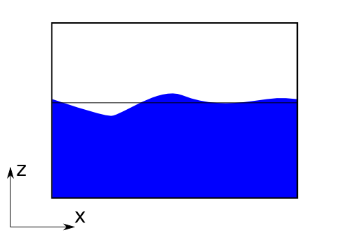
    To further simplify our problem we assume that the motion of the free surface is so small that we do not make a large error by not moving the mesh near the surface when waves travel across it. If the waves are small then the mesh points at the still water surface are sufficiently close to the actual position of the free surface that we can get away by having a constant mesh.

    Tank coordinate system

    The tank with free surface and still water water surface marked

    We need to apply linear free surface boundary conditions to get away with not moving the mesh. A quick overview of the linear free surface boundary conditions can be found for example on the Wikipedia page for Airy wave theory.

    The free surface introduces a new unknown function, \(\eta(x,t)\) in addition to the velocity potential \(\phi\). This is the surface elevation, and in our simple problem the surface elevation is only a function of the x-position in the tank and the time, t.

    The linear kinematic free surface boundary condition says that the free surface moves up and down with the velocity of the fluid at the free surface. Particles on the free surface stay on the free surface.

    \begin{equation*} \newcommand{\dif}{\mathrm{d}} \newcommand{\pdiff}[2]{\frac{\mathrm\partial#1}{\mathrm\partial#2}} \newcommand{\laplace}[1]{\nabla^2#1} \pdiff{\eta}{t} = \pdiff{\phi}{z} \quad \text{at the free surface} \end{equation*}

    The z-derivative of the velocity potential is equal to the vertical fluid speed as described in the previous blog post.

    The dynamic free surface boundary condition is derived from Bernoulli's equation and makes sure the pressure at the free surface is constant. We assume that the atmospheric pressure is zero:

    \begin{equation*} \pdiff{\phi}{t} + g\eta = 0 \quad \text{at the free surface} \end{equation*}

    We also need to specify that there is no motion through the floor of the tank:

    \begin{equation*} \pdiff{\phi}{z} = 0 \quad \text{at the the bottom} \end{equation*}

    And finally we want to move the tank back and forth to produce some free surface motion. We do this by introducing a horizontal velocity \(U_H(t)\) on the walls:

    \begin{equation*} \pdiff{\phi}{x} = U_H(t) \quad \text{on the walls} \end{equation*}

    One nice property of our equation system is that only our free surface boundary conditions involve time, the Laplace equation in the domain itself is independent of what happened at the last time step.

    Solution algorithm

    From the above we can decide on the following way to make a simulator for this problem:

    1. We need a Laplace solver that can calculate the velocity potential given a position of the free surface and a wall velocity, \(U_H\). We specify the value of the velocity potential at the free surface by using the dynamic free surface boundary condition.
    2. We need to update the free surface height function \(\eta(x,t)\) by using the kinematic free surface condition.
    3. We need to advance our solution in time and run the above in a loop.

    For point 1 we can use the previously shown FEniCS Laplace solver, with some small modifications. For point 2 we need to find a way to get the vertical derivative of the velocity potential at the free surface. For the last point we will use the built in time integration routines in SciPy so that we do not have to worry about selecting an appropriately small time step.

    We will not apply any filtering of high frequent noise on the free surface function \(\eta\), something which is common to do in Laplace equation solvers with a free surface. We will hence need a quite fine time step to avoid numerical problems. The SciPy routines have automatic time step control which avoids this problem by reducing the time step when noise is trying to sneak in. This simplification in the implementation makes our code a bit slower that it could have been.

    For the purpose of time stepping we define \(2 N\) unknowns, where \(N\) is the number of vertices on the free surface. The first half of the unknowns are the free surface elevations, while the second half is the velocity potential at the free surface:

    \begin{align*} \pdiff{\eta}{t} &= \pdiff{\phi}{z} &\qquad \text{At each of the N free surface vertices}\\ \pdiff{\phi}{t} &= - g\eta &\qquad \text{At each of the N free surface vertices} \end{align*}

    We take the initial velocity potential to be zero throughout the domain and the surface elevation is also zero at the start of the simulation.

    Derivatives

    Finding derivatives of the computed unknown function is covered in the FEniCS tutorial. Basically you can find the derivative \(w\) of the unknown function \(u\) by solving:

    \begin{equation*} w = \pdiff{u}{t} \end{equation*}

    which has the following weak form

    \begin{equation*} \int_\Omega w\,v\,\dif \Omega = \int_\Omega \pdiff{u}{t}\,v\,\dif \Omega \end{equation*}

    This can be written as follows in FEniCS:

    # The z-derivative or the velocity potential
    u2 = df.TrialFunction(V)
    v2 = df.TestFunction(V)
    a2 = u2*v2*df.dx
    L2 = df.Dx(phi, 1)*v2*df.dx
    

    This allows us to solve for the z-derivative of the solution, phi, in the whole domain. We only really need the derivative at the free surface, but for this demo I did not bother to spend time to figure out how do that.

    Code

    The complete code is available from here. I have tried to comment the code well so I hope it is relatively understandable, at least after reading these two blog posts.

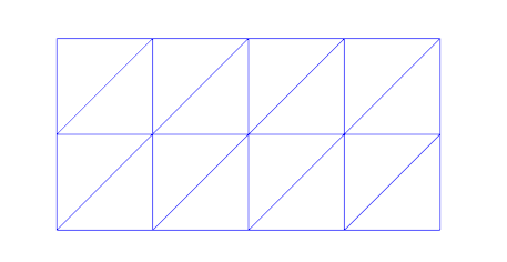
    If you look carefully you will see that the mesh has been slightly changed from the last post. The diagonals of the triangular elements are now alternating to left and right. Since the problem is highly symmetric this seemed to give significantly better results, at least for the test case I used while developing the code. Testing with higher order elements and quadrilaterals instead of triangles would be interesting, but has not been done.

    At resonance the solution does not converge, the motion amplitudes are growing linearly with time, which is expected. Below I have shown surface elevation amplitudes as function of the excitation frequency. It is simply the elevation amplitude in the last oscillation cycle that is shown, so the results around resonances depend on how many oscillations have been run. Some damping could be added to the free surface boundary condition to get converged results.

    Some results

    The results for a selected test case can be seen below in terms of surface elevation and the velocity potential:

    Free surface elevation

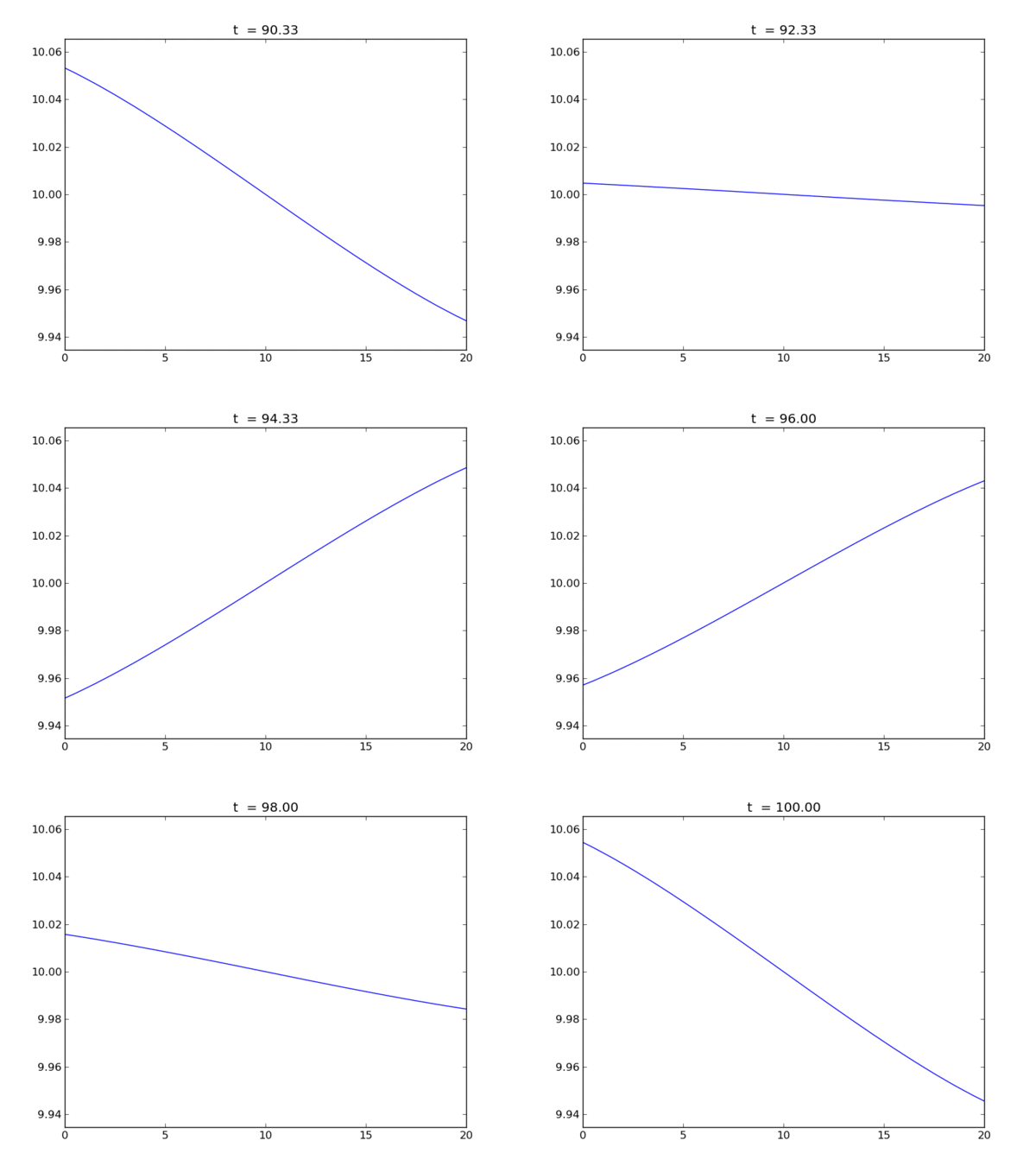
    Animation of the free surface elevation

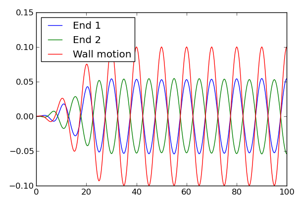
    Free surface elevation time series

    Elevation at each end of the tank as a function of time

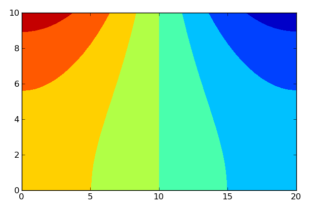
    Velocity potential

    Snapshot of the velocity potential at t=100

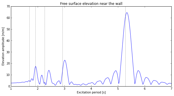
    A series of simulations were performed and the amplitudes of the free surface motion close to the walls was extracted. The results can be seen below. The resonant periods calculated by analytical formula have also been added for comparison:

    RAO for free surface elevation

    Transfer function for free surface elevation at the walls. Elevation amplitude divided by the forced motion amplitude.

    Analytical natural frequencies can be found from the following formula [Faltinsen09]:

    \begin{equation*} \omega_n = \sqrt{g\,k_n\,\tanh(k_n\,h)} \end{equation*}

    where \(k_n = n \pi / L\). The mode number is \(n\) where 1 gives the first natural mode, corresponding to a standing half sine wave. The dimensions involved are the length \(L\) and the height of the tank, \(h\).

    The calculations can be seen to be predicting roughly the physics they are intended to, but for high frequent motion the resulting velocity potential is not captured well by the selected discretization and these results are probably not very reliable.

    Calculating the above transfer function with 300 excitation periods and 20 oscillations for each period on a 40 by 20 mesh with linear triangle elements took more that 12 hours on my laptop. For this specific problem it would probably take much less time to look up and implement the analytical solution, which is not terribly hard to do. The accuracy would also be much better.

    I expect that the results given in the plot above are quite unreliable. This could easily be verified by comparing to the analytical solution, but I have not bothered with this here, as the intention was to test FEniCS for a simple dynamic problem, not promote a hopelessly inefficient method of analyzing linear sloshing in a rectangular tank.

    I do, however, believe that the method presented can be made sufficiently accurate with the right mesh and/or higher order elements and perhaps more carefull treatment of the derivative of the velocity potential on the free surface. It is then possible to incorporate nonlinear free surface boundary conditions, find solutions for non-regular tank geometries and in general quite easily find answers to questions that are very hard to find by analytical work only.

    I hope you have found this and the previous article usefull. I will probably restrict myself to smaller, bite sized, chunks if I am to continue with these posts. The topic of this article took more than one evening to code and write, and I am not sure I will devode that much time to this blog in the future. There is simply too much else to do and so many things to learn! Explaining something is still a great way to learn, so we will see if there is a follow up. Maybe the same problem, just with a discontinous Galerkin implementation instead of a continous? Time will tell.

    [Faltinsen09]Faltinsen, OM and AN Timokha, Sloshing, Cambridge University Press, 2009
  5. Solving the Laplace equation with FEniCS

    I have found that explaining something is a good way to learn. As I am currently reading some books on the finite element method to refresh my rusting memories from math courses at university I thought it would be a good idea to write a summary of some of the basics. This post will explain how to use the finite element method and FEniCS for solving partial differential equations. FEniCS is a collection of tools for automated, efficient solution of partial differential equations using the finite element method.

    Introduction

    I will show how to apply FEniCS to a simple partial differential equation. I will also explain the solution method employed in the finite element method to solve the selected equation, the Laplace equation:

    \begin{equation*} \newcommand{\dif}{\mathrm{d}} \newcommand{\pdiff}[2]{\frac{\mathrm\partial#1}{\mathrm\partial#2}} \newcommand{\laplace}[1]{\nabla^2#1} \laplace{\phi} = 0 \end{equation*}

    When a fluid is incompressible, inviscid and the flow can be assumed to be irrotational then the Laplace equation shown above describes the fluid flow. The fluid velocities, \({\bf U} = (U_x, U_y, U_z)\), can be calculated from the velocity potential \(\phi\) as follows:

    \begin{equation*} U_x = \pdiff{\phi}{x} \qquad U_y = \pdiff{\phi}{x} \qquad U_z = \pdiff{\phi}{x} \end{equation*}

    Our domain, \(\Omega\), is a 2D square with \(x \in [0, 2]\) and \(y \in [0, 1]\). For the boundary conditions, let's say that we know the value of \(\phi\) at that the short boundaries and the normal derivative at the long edges is zero. The complete equation system can then be for example:

    \begin{align*} &\laplace{\phi} = 0 \\ \ \\ &\phi = -1.0 \quad &\text{on} \quad x = 0.0 \\ &\phi = +1.0 \quad &\text{on} \quad x = 2.0 \\ &\pdiff{\phi}{\bf n} = 42 \quad &\text{on} \quad \Gamma_L \\ \end{align*}

    where we define \(\Gamma_L\) to be the long edge boundaries \(y=0\) and \(y=1\). The normal vector on the boundary is \(\bf n\) and \(\pdiff{}{\bf n}\) is the normal derivative at the boundary. It is common to use \(\Omega\) to denote the domain and \(\Gamma\) to denote the boundary.

    Discretization

    Now, to solve the equation with boundary conditions we need a discretized domain. This can be created by using the FEniCS Python package dolfin like this:

    import dolfin as df
    
    start_x, end_x, n_elem_x = 0.0, 2.0, 4
    start_y, end_y, n_elem_y = 0.0, 1.0, 2
    
    mesh = df.RectangleMesh(start_x, start_y, end_x, end_y, n_elem_x, n_elem_y)
    

    Running df.plot(mesh) will show the following:

    The mesh

    An example mesh with triangular elements

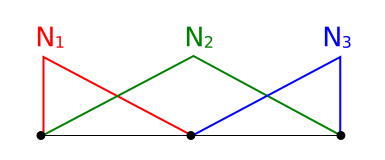
    We discretize our domain \(\Omega\) into discrete elements and obtain \(\hat \Omega\). I will use the "hat" to denote discretized values. We use linear elements which means we will approximate the unknown function with piecewise linear functions, \(\phi \approx \hat \phi\). They look like this for a 1D domain with two elements and three vertices (nodes):

    Linear shape functions in 1D

    1D domain with three shape functions, \(N_1(x)\), \(N_2(x)\) and \(N_3(x)\)

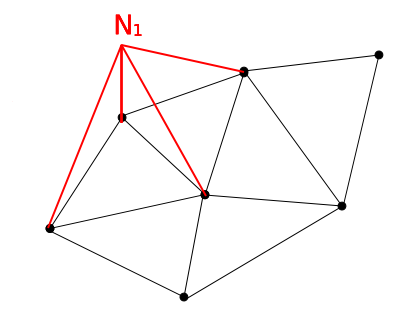
    We have one shape function \(N_i\) for each vertex in the mesh. The shape functions are equal to 1.0 at the corresponding vertex and 0.0 at all other vertices. In 2D a standard bi-linear shape function looks as follows:

    Linear shape function in 2D

    2D domain with a bi-linear shape function shown for one of the vertices on the boundary

    Marking the boundaries

    We know how to make a mesh of the domain. We also need to tell FEniCS about the different parts of the boundary. We do this by giving the boundaries different unique integer numbers and marking the boundaries with a mesh function:

    # Each part of the mesh gets its own ID
    ID_LEFT_SIDE, ID_RIGHT_SIDE, ID_BOTTOM, ID_TOP, ID_OTHER = 1, 2, 3, 4, 5
    boundary_parts = df.MeshFunction("size_t", mesh, mesh.topology().dim()-1)
    boundary_parts.set_all(ID_OTHER)
    
    # Define the boundaries
    GEOM_TOL = 1e-6
    define_boundary(lambda x, on_boundary: on_boundary and x[0] < start_x + GEOM_TOL, boundary_parts, ID_LEFT_SIDE)
    define_boundary(lambda x, on_boundary: on_boundary and x[0] > end_x - GEOM_TOL, boundary_parts, ID_RIGHT_SIDE)
    define_boundary(lambda x, on_boundary: on_boundary and x[1] < start_y + GEOM_TOL, boundary_parts, ID_BOTTOM)
    define_boundary(lambda x, on_boundary: on_boundary and x[1] > end_y - GEOM_TOL, boundary_parts, ID_TOP)
    

    The define_boundary function is just a small utility I made to make it easier to mark the boundaries. Normally you need to create a class for each boundary and implement a method, inside, on this class. My function accepts a lambda expression which is used instead:

    def define_boundary(defining_func, boundary_parts, boundary_id):
        """
        Define a boundary
    
        - defining_func is used instead of the normal SubDomain inside method: defining_func(x, on_boundary)
        - boundary_parts is a MeshFunction used to distinguish parts of the boundary from each other
        - boundary_id is the id of the new boundary in the boundary_parts dictionary
        """
        class Boundary(df.SubDomain):
            def inside(self, x, on_boundary):
                return defining_func(x, on_boundary)
        boundary = Boundary()
        boundary.mark(boundary_parts, boundary_id)
        return boundary
    

    The solution method

    The simplest variant of the finite element method to describe is probably the Galerkin weighted residuals method. The core of the method is described below.

    The unknown function \(\phi\) is written as a sum of \(M\) shape functions and a set of unknown coefficients, \(a_i\). There is one unknown coefficient for each shape function:

    \begin{equation*} \hat \phi(x,y) = \sum_{i=0}^{M} a_i N_i(x,y) \end{equation*}

    Suppose we guess some coefficients \(a_i\). We can then integrate our trial function, \(\hat \phi\) over the domain, but since the discretization is not perfect we get a residual and not zero as the equation was supposed to give:

    \begin{equation*} \int_{\Omega} \laplace{\hat \phi} \ \dif \Omega = R \end{equation*}

    To be able to fix this and find some coefficients \(a_i\) that gives zero residual we need a set of equations. This is done by multiplying the above integral with a set of weighing functions, \(w_i(x,y)\). The number of weighting functions is equal to the number of unknowns, so we get a fully determined set of linear equations. In the Galerkin method the weighting functions are taken equal to the shape functions, \(N_i\) except that we do not include shape functions corresponding to vertices where we know the solution \(\phi(x,y)\) from the Dirichlet boundary conditions.

    We then get a set of \(M\) equations:

    \begin{equation*} \int_{\Omega} \laplace{\hat \phi} w_i \ \dif \Omega = 0 \end{equation*}

    which is the same as:

    \begin{equation*} \int_{\Omega} \laplace{\left(\sum_{j=0}^M a_j N_j\right)} N_i \dif \Omega = 0 \end{equation*}

    Since the integral will only be non-zero for vertices that are close in the mesh, i.e. \(N_i\) and \(N_j\) have some overlap, we end up with a quite sparse equation system. Very efficient solvers exist for the types of equation systems that come out of the Galerkin method.

    Solving the equation system with FEniCS

    In the standard finite element terminology our unknown function \(\phi\) is called the trial function and denoted \(u\) while the weighting function is called the test function and denoted \(v\). We switch to this terminology to be compatible with the FEniCS tutorial. We call this equation the weak form:

    \begin{equation*} \int_{\Omega} \laplace{(u)}\,v \ \dif \Omega = 0 \end{equation*}

    Before we are done we need to modify the equation a bit. As written it makes little sense since the Laplacian of the bi-linear function \(N_j(x,y)\) will always be zero. We modify our weak form by performing integration by parts. The formula for this in higher dimensions is:

    \begin{equation*} \int_\Omega \pdiff{f}{x_i}\,g \ \dif \Omega = \int_\Gamma f\,g\,n_i\ \dif \Gamma - \int_\Omega f \pdiff{g}{x_i} \ \dif \Omega \end{equation*}

    where \(n_i\) is the \(i\)-th component of the outwards normal vector on \(\Gamma\). I do not think I ever learned that at school? Maybe it's just my rusty memory, but thanks to Wikipedia we will not let lacking education and/or failing memory stop us, now will we? We get this when applying integration by parts to our integral:

    \begin{equation*} \int_\Omega \laplace{(u)}\,v \ \dif \Omega = \int_\Gamma \nabla(u)\,v\,n_i\ \dif \Gamma - \int_\Omega \nabla (u)\cdot\nabla(v) \ \dif \Omega \end{equation*}

    I guess now is the time for me to remember to mention that the test function \(v\) is always zero at the Dirichlet boundaries. Dirichlet boundaries are boundaries where we have Dirichlet boundary conditions, which means we know the value of \(\phi\), i.e. the short edges of our mesh in this case. No reason to have a weight function there, right? We now have the final expression for the weak form:

    \begin{align*} \int_{\Omega} \nabla u \cdot \nabla v \ \dif \Omega &= \int_{\Gamma_N} \laplace{(u)}\,v\,n_i\ \dif \Gamma_N \\ &= \int_{\Gamma_N} \pdiff{u}{\bf n}\,v\ \dif \Gamma_N \end{align*}

    The long edges were we prescribe the normal velocity (normal derivative of the velocity potential \(\phi\)) are now denoted \(\Gamma_N\) since this type of boundary condition is called a Neumann boundary condition.

    FEniCS understands equations such as the above and calls them forms. To describe the equations we use UFL, Uniform Form Language which is a Python API for defining forms. When interacting with FEniCS through Python we can use UFL through the dolfin package just like the mesh facilities. UFL can also be directly imported, import ufl.

    # Define a function space of bi-linear elements on our mesh
    V = df.FunctionSpace(mesh, 'Lagrange', 1)
    
    # The trial and test functions are defined on the bi-linear function space
    u = df.TrialFunction(V)
    v = df.TestFunction(V)
    
    # Our equation is defined as a=L. We only define what is inside the integrals, and the difference
    # between integrals over the domain and the boundary is whether we use dx or ds:
    #   - the term a contains both the trial (unknown) function u and the test function v
    #   - the term L contains only test function v
    a = df.inner(df.nabla_grad(u), df.nabla_grad(v))*df.dx
    L = df.Constant(42)*v*df.ds(ID_BOTTOM) + df.Constant(42)*v*df.ds(ID_TOP)
    

    This is basically all there is to solving the Laplace equation in FEniCS. The complete code can be seen below. The parts I have skipped explaining above are well explained in the FEniCS tutorial.

    Complete code

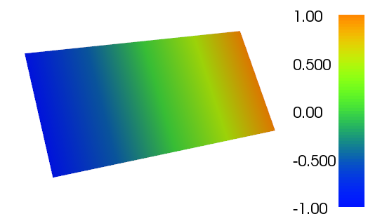
    The complete code can be found on Bitbucket. The resulting plot from running the code with FEniCS 1.3 is shown below:

    Plot of the result

    Plot of the resulting \(\phi\) function

    If you have any questions to the above and how to use FEniCS you can ask here, but I would really recommend the FEniCS QA Forum where you will probably get better and faster answers.

Page 1 / 2 »