Tormod Landet

In the previous blog post I showed how to solve the Laplace equation in 2D with FEniCS. That example, while illustrative for how to use FEniCS, was not particularly exciting. So, I decided to show the simplest example I could think of that involves an actual example of fluid flow.

Before we start: Writing these posts is a learning exercise for me. If you are learning FEniCS or the finite element method, please do not consider this material authoritative. I still hope this can be useful for someone else, but correctness is not guaranteed. In addition no mesh sensitivity studies or rigorous validation has been performed. This work has been done in evenings when I have felt like it, and then producing something that is much more fun than carefully testing it afterwards. Just so you know before we start on the real content of this post.

Sloshing

Sloshing is the motion of a fluid with a free surface in an enclosed space, such as a tank or a glass of water. The term free surface simply means the top of the fluid is allowed to move freely.

The simplest way to simulate sloshing with FEniCS is with a 2D rectangular tank and incompressible, irrotational and inviscid fluid flow. This is called potential flow and we only need to solve the Laplace equation for the scalar velocity potential, normally called \(\phi\), and not the velocities and the pressure which can be calculated from the derivatives of the velocity potential function. This makes potential flow solvers fast, and hence popular, but of course not applicable to all problems of fluid flow!

\begin{equation*} \newcommand{\dif}{\mathrm{d}} \newcommand{\pdiff}[2]{\frac{\mathrm\partial#1}{\mathrm\partial#2}} \newcommand{\laplace}[1]{\nabla^2#1} \laplace{\phi} = 0 \qquad \text{(the Laplace equation)} \end{equation*}

To further simplify our problem we assume that the motion of the free surface is so small that we do not make a large error by not moving the mesh near the surface when waves travel across it. If the waves are small then the mesh points at the still water surface are sufficiently close to the actual position of the free surface that we can get away by having a constant mesh.

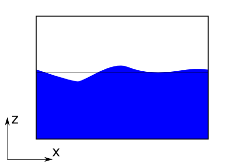
The tank with free surface and still water water surface marked

We need to apply linear free surface boundary conditions to get away with not moving the mesh. A quick overview of the linear free surface boundary conditions can be found for example on the Wikipedia page for Airy wave theory.

The free surface introduces a new unknown function, \(\eta(x,t)\) in addition to the velocity potential \(\phi\). This is the surface elevation, and in our simple problem the surface elevation is only a function of the x-position in the tank and the time, t.

The linear kinematic free surface boundary condition says that the free surface moves up and down with the velocity of the fluid at the free surface. Particles on the free surface stay on the free surface.

\begin{equation*} \newcommand{\dif}{\mathrm{d}} \newcommand{\pdiff}[2]{\frac{\mathrm\partial#1}{\mathrm\partial#2}} \newcommand{\laplace}[1]{\nabla^2#1} \pdiff{\eta}{t} = \pdiff{\phi}{z} \quad \text{at the free surface} \end{equation*}

The z-derivative of the velocity potential is equal to the vertical fluid speed as described in the previous blog post.

The dynamic free surface boundary condition is derived from Bernoulli's equation and makes sure the pressure at the free surface is constant. We assume that the atmospheric pressure is zero:

\begin{equation*} \pdiff{\phi}{t} + g\eta = 0 \quad \text{at the free surface} \end{equation*}

We also need to specify that there is no motion through the floor of the tank:

\begin{equation*} \pdiff{\phi}{z} = 0 \quad \text{at the the bottom} \end{equation*}

And finally we want to move the tank back and forth to produce some free surface motion. We do this by introducing a horizontal velocity \(U_H(t)\) on the walls:

\begin{equation*} \pdiff{\phi}{x} = U_H(t) \quad \text{on the walls} \end{equation*}

One nice property of our equation system is that only our free surface boundary conditions involve time, the Laplace equation in the domain itself is independent of what happened at the last time step.

Solution algorithm

From the above we can decide on the following way to make a simulator for this problem:

We need a Laplace solver that can calculate the velocity potential given a position of the free surface and a wall velocity, \(U_H\). We specify the value of the velocity potential at the free surface by using the dynamic free surface boundary condition.
We need to update the free surface height function \(\eta(x,t)\) by using the kinematic free surface condition.
We need to advance our solution in time and run the above in a loop.

For point 1 we can use the previously shown FEniCS Laplace solver, with some small modifications. For point 2 we need to find a way to get the vertical derivative of the velocity potential at the free surface. For the last point we will use the built in time integration routines in SciPy so that we do not have to worry about selecting an appropriately small time step.

We will not apply any filtering of high frequent noise on the free surface function \(\eta\), something which is common to do in Laplace equation solvers with a free surface. We will hence need a quite fine time step to avoid numerical problems. The SciPy routines have automatic time step control which avoids this problem by reducing the time step when noise is trying to sneak in. This simplification in the implementation makes our code a bit slower that it could have been.

For the purpose of time stepping we define \(2 N\) unknowns, where \(N\) is the number of vertices on the free surface. The first half of the unknowns are the free surface elevations, while the second half is the velocity potential at the free surface:

\begin{align*} \pdiff{\eta}{t} &= \pdiff{\phi}{z} &\qquad \text{At each of the N free surface vertices}\\ \pdiff{\phi}{t} &= - g\eta &\qquad \text{At each of the N free surface vertices} \end{align*}

We take the initial velocity potential to be zero throughout the domain and the surface elevation is also zero at the start of the simulation.

Derivatives

Finding derivatives of the computed unknown function is covered in the FEniCS tutorial. Basically you can find the derivative \(w\) of the unknown function \(u\) by solving:

\begin{equation*} w = \pdiff{u}{t} \end{equation*}

which has the following weak form

\begin{equation*} \int_\Omega w\,v\,\dif \Omega = \int_\Omega \pdiff{u}{t}\,v\,\dif \Omega \end{equation*}

This can be written as follows in FEniCS:

# The z-derivative or the velocity potential
u2 = df.TrialFunction(V)
v2 = df.TestFunction(V)
a2 = u2*v2*df.dx
L2 = df.Dx(phi, 1)*v2*df.dx

This allows us to solve for the z-derivative of the solution, phi, in the whole domain. We only really need the derivative at the free surface, but for this demo I did not bother to spend time to figure out how do that.

Code

The complete code is available from here. I have tried to comment the code well so I hope it is relatively understandable, at least after reading these two blog posts.

If you look carefully you will see that the mesh has been slightly changed from the last post. The diagonals of the triangular elements are now alternating to left and right. Since the problem is highly symmetric this seemed to give significantly better results, at least for the test case I used while developing the code. Testing with higher order elements and quadrilaterals instead of triangles would be interesting, but has not been done.

At resonance the solution does not converge, the motion amplitudes are growing linearly with time, which is expected. Below I have shown surface elevation amplitudes as function of the excitation frequency. It is simply the elevation amplitude in the last oscillation cycle that is shown, so the results around resonances depend on how many oscillations have been run. Some damping could be added to the free surface boundary condition to get converged results.

Some results

The results for a selected test case can be seen below in terms of surface elevation and the velocity potential:

Animation of the free surface elevation

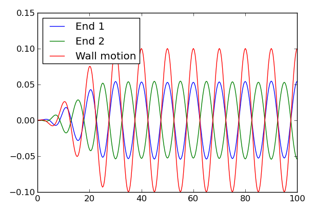
Elevation at each end of the tank as a function of time

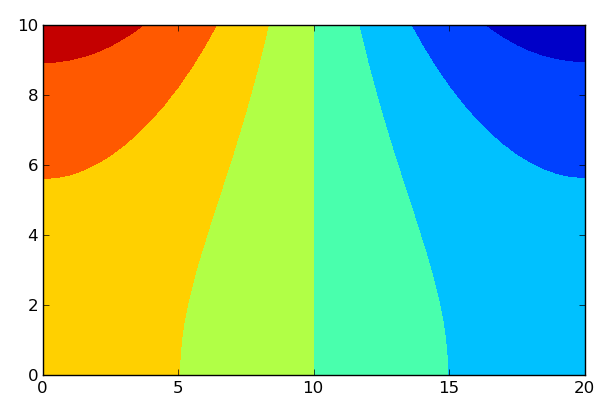
Snapshot of the velocity potential at t=100

A series of simulations were performed and the amplitudes of the free surface motion close to the walls was extracted. The results can be seen below. The resonant periods calculated by analytical formula have also been added for comparison:

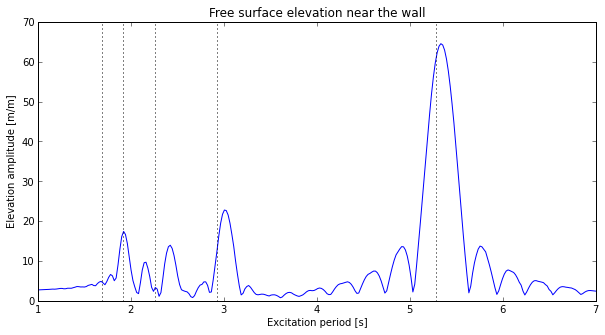
Transfer function for free surface elevation at the walls. Elevation amplitude divided by the forced motion amplitude.

Analytical natural frequencies can be found from the following formula [Faltinsen09]:

\begin{equation*} \omega_n = \sqrt{g\,k_n\,\tanh(k_n\,h)} \end{equation*}

where \(k_n = n \pi / L\). The mode number is \(n\) where 1 gives the first natural mode, corresponding to a standing half sine wave. The dimensions involved are the length \(L\) and the height of the tank, \(h\).

The calculations can be seen to be predicting roughly the physics they are intended to, but for high frequent motion the resulting velocity potential is not captured well by the selected discretization and these results are probably not very reliable.

Calculating the above transfer function with 300 excitation periods and 20 oscillations for each period on a 40 by 20 mesh with linear triangle elements took more that 12 hours on my laptop. For this specific problem it would probably take much less time to look up and implement the analytical solution, which is not terribly hard to do. The accuracy would also be much better.

I expect that the results given in the plot above are quite unreliable. This could easily be verified by comparing to the analytical solution, but I have not bothered with this here, as the intention was to test FEniCS for a simple dynamic problem, not promote a hopelessly inefficient method of analyzing linear sloshing in a rectangular tank.

I do, however, believe that the method presented can be made sufficiently accurate with the right mesh and/or higher order elements and perhaps more carefull treatment of the derivative of the velocity potential on the free surface. It is then possible to incorporate nonlinear free surface boundary conditions, find solutions for non-regular tank geometries and in general quite easily find answers to questions that are very hard to find by analytical work only.

I hope you have found this and the previous article usefull. I will probably restrict myself to smaller, bite sized, chunks if I am to continue with these posts. The topic of this article took more than one evening to code and write, and I am not sure I will devode that much time to this blog in the future. There is simply too much else to do and so many things to learn! Explaining something is still a great way to learn, so we will see if there is a follow up. Maybe the same problem, just with a discontinous Galerkin implementation instead of a continous? Time will tell.

[Faltinsen09]

Faltinsen, OM and AN Timokha, Sloshing, Cambridge University Press, 2009

Articles tagged with Sloshing

A linear 2D sloshing solver in FEniCS

Sloshing

Solution algorithm

Derivatives

Code

Some results

Sommerferie / Master of Science